[Kaggle] TPSMAR22, Temporal Fusion Transform 써보기(Private 4등!!!)

이 글이 도움되셨다면 광고 클릭 부탁드립니다 : )

캐글에서 Tabular Playground Series라고 캐글 초보자들을 위한 Tabular 형식의 데이터 분석 과제를 매 달 만들어 주고 있습니다. playground series는 캐글의 다른 대회와는 성격이 조금 다른데, Tabular 데이터를 제공해 누구나 접근할 수 있는 문제를 제시하여 비기너들이 학습하고 성장하는 것을 목표로 합니다.
그래서 타 대회는 상금이 있는 반면, TPS는 상위 3개 팀에게 Kaggle Merchandise를 줍니다.
저도 언젠가 받을 수 있겠죠...?

아직 진행 중이지만, 추후 코드/아이디어 재활용을 위한 기록을 남겨봅니다.

 

---

 

0. TPSMAR22

3월 TPS에서는 미국의 도로 정체를 예측하는 과제를 풀게 됩니다.
https://www.kaggle.com/c/tabular-playground-series-mar-2022/overview

Tabular Playground Series - Mar 2022 | Kaggle

제공되는 정보는 시간, 도로의 위치 정보, 도로의 방향 그리고 우리가 예측해야 하는 congestion 변수가 nomalize되어있습니다.

row_id - a unique identifier for this instance
time - the 20-minute period in which each measurement was taken
x - the east-west midpoint coordinate of the roadway
y - the north-south midpoint coordinate of the roadway
direction - the direction of travel of the roadway.
congestion - congestion levels for the roadway during each hour; the target. The congestion measurements have been normalized to the range 0 to 100.

Train 데이터는 1991년 4월 1일 00시 20분부터 1991년 9월 30일 11시 40분까지 도로 정체 정보로 그 이후 시간인 1991년 9월 30일 12시 00분부터 1991년 9월 30일 23시 40분까지의 도로 정체 정도를 예측하면 됩니다.

row_id	time	x	y	direction	congestion
0	1991-04-01 00:00:00	0	0	EB	70
1	1991-04-01 00:00:00	0	0	NB	49

 

 

1. EDA

우선 결측없이 각 좌표와 방향 별 20분 단위로 도로 정체 수준이 수집되어 있으며 좌표와 방향 별 도로 정체 분포가 다른 것을 확인할 수 있습니다.

# count plot
fig, axes = plt.subplots(1,3, figsize=(30,10))
sns.countplot(x='x', data=train, ax=axes[0], palette='Set2')
sns.countplot(x='y', data=train, ax=axes[1], palette='Set2')
sns.countplot(x='direction', data=train, ax=axes[2], palette='Set2')

# displot
sns.displot(train.congestion, kind='hist', kde=True, color=sns.color_palette("Set2")[0])
# displot by condition
fig, axes = plt.subplots(4,3, figsize=(30,15))
plt.setp(axes, xlim=(0,100), ylim=(0,14000))
for i in range(3):
    for j in range(4):
        sns.histplot(train[(train.x==i)&(train.y==j)].congestion,  kde=True, ax = axes[j][i], color=sns.color_palette("Set2")[0])

# violinplot
fig, axes = plt.subplots(1,3, figsize=(30,10))
sns.violinplot(x='x', y='congestion', data=train, ax=axes[0], palette='Set2')
sns.violinplot(x='y', y='congestion', data=train, ax=axes[1], palette='Set2')
sns.violinplot(x='direction', y='congestion', data=train, ax=axes[2], palette='Set2')

 

다음은 시간 변수에 대한 특징을 알아보기 위해 간단히 prophet 돌려보니(코드참고) holiday나 weekly, daily 패턴이 확실히 보였습니다.

아래 주황색 bar는 각각 Memorial day, Independence day, labor day로 공휴일에는 도로 정체가 감소하는 경향을 보입니다.

# barplot
fig = plt.figure(figsize=(30,10))
sns.barplot(data=train_time_date, x='ds',y='y',hue='holiday_yn', palette=sns.color_palette("Set2")[:2])
plt.xticks(rotation=90)

 

 

2. Feature Engineering

제공되는 변수만으로는 한계가 있어 타 노트북 참고하여 다양한 변수를 생성해줍니다.

def feature_engineering(data):
    data['time'] = pd.to_datetime(data['time'])
    data['month'] = data['time'].dt.month
    data['weekday'] = data['time'].dt.weekday
    data['hour'] = data['time'].dt.hour
    data['minute'] = data['time'].dt.minute
    data['holiday_yn'] = np.where(data.time.dt.date.isin(holidays),1,0).astype('str')
    data['converted_direction_coord_0'] = data['direction'].map(lambda x: dir_mapper[x][0])
    data['converted_direction_coord_1'] = data['direction'].map(lambda x: dir_mapper[x][1])
    data['is_month_start'] = data['time'].dt.is_month_start.astype('int')
    data['is_month_end'] = data['time'].dt.is_month_end.astype('int')
    data['hour+minute'] = data['time'].dt.hour * 60 + data['time'].dt.minute
    data['is_weekend'] = (data['time'].dt.dayofweek > 4).astype('int')
    data['is_afternoon'] = (data['time'].dt.hour > 12).astype('int')
    data['x+y'] = data['x'].astype('str') + data['y'].astype('str')
    data['x+y+direction'] = data['x'].astype('str') + data['y'].astype('str') + data['direction'].astype('str')
    data['x+y+direction0'] = data['x'].astype('str') + data['y'].astype('str') + data['converted_direction_coord_0'].astype('str')
    data['x+y+direction1'] = data['x'].astype('str') + data['y'].astype('str') + data['converted_direction_coord_1'].astype('str')
    data['hour+direction'] = data['hour'].astype('str') + data['direction'].astype('str')
    data['hour+x+y'] = data['hour'].astype('str') + data['x'].astype('str') + data['y'].astype('str')
    data['hour+direction+x'] = data['hour'].astype('str') + data['direction'].astype('str') + data['x'].astype('str')
    data['hour+direction+y'] = data['hour'].astype('str') + data['direction'].astype('str') + data['y'].astype('str')
    data['hour+direction+x+y'] = data['hour'].astype('str') + data['direction'].astype('str') + data['x'].astype('str') + data['y'].astype('str')
    data['hour+x'] = data['hour'].astype('str') + data['x'].astype('str')
    data['hour+y'] = data['hour'].astype('str') + data['y'].astype('str')

for data in [train, test]:
    feature_engineering(data)

medians = pd.DataFrame(train.groupby(['x+y+direction', 'weekday', 'hour', 'minute']).congestion.median().astype(int)).reset_index()
medians = medians.rename(columns={'congestion':'median'})
train = train.merge(medians, on=['x+y+direction', 'weekday', 'hour', 'minute'], how='left')
test = test.merge(medians, on=['x+y+direction', 'weekday', 'hour', 'minute'], how='left')

mins = pd.DataFrame(train.groupby(['x+y+direction', 'weekday', 'hour', 'minute']).congestion.min().astype(int)).reset_index()
mins = mins.rename(columns={'congestion':'min'})
train = train.merge(mins, on=['x+y+direction', 'weekday', 'hour', 'minute'], how='left')
test = test.merge(mins, on=['x+y+direction', 'weekday', 'hour', 'minute'], how='left')

maxs = pd.DataFrame(train.groupby(['x+y+direction', 'weekday', 'hour', 'minute']).congestion.max().astype(int)).reset_index()
maxs = maxs.rename(columns={'congestion':'max'})
train = train.merge(maxs, on=['x+y+direction', 'weekday', 'hour', 'minute'], how='left')
test = test.merge(maxs, on=['x+y+direction', 'weekday', 'hour', 'minute'], how='left')

 

 

3. Temporal Fusion Transform

사실 Temporal Fusion Transform(논문)가 정확하게 어떤 구조를 가지는 지는 모른 채 지인의 추천을 받아 적용해보았습니다.

Illustration of multi-horizon forecasting with static covariates, past-observed and apriori-known future time-dependent inputs.

TFT 모델은 2019년 구글에서 발표한 시계열계의 SOTA 알고리즘이라고 합니다. 단순 목적 변수만 가지고 예측하는 전통적인 시계열 예측 방법(단변량 방법론, ARIMA...)에서 나아가 미래이지만 시간과 상관없이 우리가 알고 있는 정보(static covariates)를 함께 활용하여 예측 성능을 높였습니다.

TPSMAR22에서도 단독 모델로 성능이 좋았고, MAE 5.0대로 진입할 수 있었습니다.
(학습을 길게 하면 MAE가 더 떨어지긴 함)

pytorch로 구현되어 있으며 아래 튜토리얼 참고하면 간단하게 따라 해 볼 수 있습니다.
https://pytorch-forecasting.readthedocs.io/en/stable/tutorials/stallion.html

Demand forecasting with the Temporal Fusion Transformer — pytorch-forecasting  documentation

TFT 모델 피팅을 위해서는 time_id를 만들어줘야 합니다.

train['time_id'] = ( ( (train.time.dt.dayofyear-1)*24*60 + train.time.dt.hour*60 + train.time.dt.minute ) /20 ).astype(int)
test['time_id'] = ( ( (test.time.dt.dayofyear-1)*24*60 + test.time.dt.hour*60 + test.time.dt.minute ) /20 ).astype(int)
prediction_steps = test['time_id'].nunique()

우리가 예측할 congestion변수 이 외에 static 한 categorical변수와 real변수를 따로 지정하거나 time-varying변수도 추가로 지정하여 모델 학습에 사용합니다.

training = TimeSeriesDataSet(
    train_tab[lambda x: x["time_id"] <= training_cutoff],
    time_idx="time_id", # 시간 인덱스 값
    target="congestion", # target 변수
    group_ids=["x+y+direction"], 
    min_encoder_length=0,  
    max_encoder_length=max_encoder_length,
    min_prediction_length=1,
    max_prediction_length=max_prediction_length,
    # list of categorical variables that do not change over time
    static_categoricals=['holiday_yn','x+y', 'x+y+direction', 'x+y+direction0','x+y+direction1'],
    # list of continuous variables that do not change over time
    static_reals=[],
    #  list of categorical variables that change over time and are known in the future
    time_varying_known_categoricals=['month', 'weekday', 'hour', 'minute','is_month_start', 'is_month_end', 'hour+minute', 'is_weekend',
       'is_afternoon','hour+direction', 'hour+x+y', 'hour+direction+x',
       'hour+direction+y', 'hour+direction+x+y', 'hour+x', 'hour+y'],  
    # list of continuous variables that change over time and are known in the future
    time_varying_known_reals=["time_id","min","max",'median'],
    #  list of continuous variables that change over time and are not known in the future. You might want to include your target here.
    time_varying_unknown_reals=["congestion"],    
    add_relative_time_idx=True,
    add_target_scales=True,
    add_encoder_length=True,
    allow_missing_timesteps=True    
 )

optuna가 내재되어 있어 하이퍼파라미터 최적화를 간단하게 진행할 수 있습니다.

from pytorch_forecasting.models.temporal_fusion_transformer.tuning import optimize_hyperparameters

# create study optuna
study = optimize_hyperparameters(
    train_dataloader,
    val_dataloader,
    model_path="optuna_test",
    n_trials=50,
    max_epochs=20,
    gradient_clip_val_range=(0.01, 1.0),
    hidden_size_range=(8, 64),
    hidden_continuous_size_range=(8, 64),
    attention_head_size_range=(1, 4),
    learning_rate_range=(0.001, 0.1),
    dropout_range=(0.1, 0.3),
    trainer_kwargs=dict(limit_train_batches=30, log_every_n_steps=15, gpus=1),
    reduce_on_plateau_patience=4,
    use_learning_rate_finder=False,  # use Optuna to find ideal learning rate or use in-built learning rate finder
    timeout=5400  # we can increase the timeout for better tuning.
)
# show best hyperparameters
print(study.best_trial.params)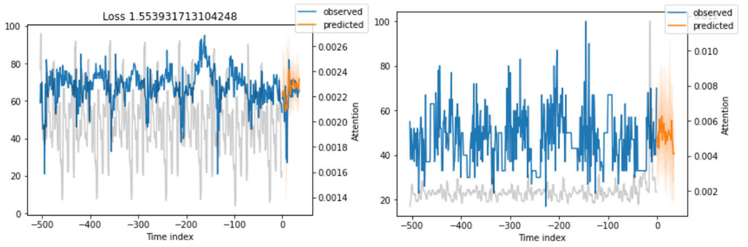

 

 

4. Calculate the average of similar day's congestion

아래 노트북은 아주 간단한 방법으로 public score 4.988을 받았는데, 컨셉은 이렇습니다.
우리가 예측해야 하는 시간은 1991년 9월 30일 오후 시간대이니까 오전 동안의 정체 수준이 비슷한 날을 골라 그날들의 위치별 방향별 평균/중앙값으로 예측하는 것입니다.

결과가 좋아서 그런지 나름 논리적이고 엄청나게 효율적이라고 생각됩니다.
보통 예측을 해야 하면 모델에 먼저 넣어보는데 이렇게 간단한 방법으로 접근해봐도 좋을 것 같습니다.
https://www.kaggle.com/horrip/tpsmar22-average-baseline-lb-4-992

TPSMAR22 Average baseline LB 4.992

 

 

Private 4등!!

어쩌다가 4등을 해버렸습니다 ㅎㅎ!
사실 그렇게 다양한 시도를 해보고 시간을 많이 쏟은게 아니라서 결과가 떴을 때 내가...? 대체 왜...? 반응이 먼저였는데 다시는 오지 않을 것 같은 결과인 만큼 박제해두도록 하겠습니다 : )
최종 모델은 위의 TFT, Tabnet, Calculate the average of similar day's congestion의 결과와 특정시간&위치의 special value를 앙상블하여 최종 결과를 냈습니다.
Entries를 보면 알 수 있겠지만 14번 밖에 제출을 안했는데 운이 좋았나봅니다.
언젠가는 어쩌다가 1등...하는 포스트를 적는 날도 오겠죠...? ㅎㅎ