[논문 리뷰] 이상치 탐지 | Deep Isolation Forest for Anomaly Detection

이 글이 도움 되셨다면 광고 클릭 부탁드립니다 : )

 

오랜만에 이상치 탐지 방법론 리뷰를 해보려고 합니다. 어떤 방법론을 공부해볼까 하고 찾아보다 2023년에 나온 Deep Isolation Forest for Anomaly Detection, DIF라는 Isolation Forest 기반의 딥러닝 방법론이 있어 살펴보려고 합니다. PyOD 라이브러리에 들어가 있어서 실제 적용도 간단하게 해 볼 수 있을 것 같네요.

https://slowsteadystat.tistory.com/25

PyOD 라이브러리로 간단하게 이상치 탐지하기

 

---

0. Isolation Forest?!

먼저 DIF리뷰에 앞서 Isolation Forest가 어떤 방법인지 가볍게 복습하고 넘어가겠습니다. 

Isolation Forest(2008)는 이상치 데이터는 적은 수의 공간분할 만으로 isolation이 가능할 것이라는 간단한 아이디어에서 생겨난  unsupervised anomaly detection 방법론입니다. 기존 거리기반이나 밀도기반의 이상치 탐지 방법론은 고차원이나 데이터가 많은 경우 성능이 떨어진다는 단점이 있는데, Isolation Forest는 거리나 밀도기반이 아니기 때문에 계산량이 적어 시간 복잡도가 낮고 고차원과 많은 데이터셋에서도 성능이 보존된다는 장점을 가집니다.

• 정상 군집에서 떨어진 데이터 $x_o$는 적은 수의 공간 분할만으로 isolation 가능
• 의사결정나무를 몇 회 타고 내려가서 고립되는 지를 기준으로 정상치와 이상치 분리

 

 

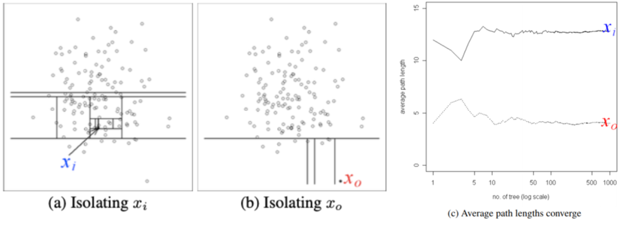
기본적인 동작 방식은 (Training)전체 데이터 중에 sub_sample을 뽑아 sub_sample내 모든 데이터가 isolation 되는 iTree들을 만들고 앙상블 하여 iForest를 만든 뒤, (Evaluation) 각 데이터가 root node에서부터 terminal node에 도달하기까지의 평균 path length를 바탕으로 anomaly score를 계산하는 방법론입니다.

 

 

1. Deep Isolation Forest for Anomaly Detection?!

1.1 Abstract

iForest가 나온 뒤로 다양한 isolation forest기반의 이상치 탐지 방법론이 나왔지만 기본 iForest가 가지는 axis-parallel isolaion이 가지는 단점(고차원/비선형 데이터에서의 한계)을 완전하게 극복하지 못했습니다. 그래서 본 논문에서는 신경망을 활용해서 원본 데이터를 axis-parallel로도 구분이 가능하도록 random representation ensemble에 맵핑하는 방법을 제안하였습니다. 이러한 random representation 방법으로 원본 데이터에서의 파티션에 대한 높은 자유도를 주고(비선형 partition도 가능하게 되어) random representation과 random partition-based isolation 간의 시너지를 낼 수 있다고 설명합니다. 

 

 

1.2 Introduction

거리/밀도기반 방법과는 달리 iForest는 "적고 다르다"(few and different) 는 이상치가 가지는 핵심 특징을 더 반영했다고 볼 수 있습니다. 더불어 시간 복잡도가 낮다는 강점에 여러 산업 분야에서 각광받고 있습니다. 반면 iForest가 가지는 한계점도 명확합니다.

 

첫 번째로는 고차원 공간(여러 피처들의 조합에서 확인되는?)에서만 isolation되는 hard anomalies를 탐지하기 어렵다는 점입니다. Fig1에서 보면 가장 왼쪽의 가상의 데이터에서 삼각형의 anomalies를 axis-parallel partition으로 분리해 낼 수가 없는데(여러 번 반복하면 isolation 되겠지만 그렇게 되면 정상 데이터와 path length 구분이 안됨), 동일한 데이터를 representation 한 오른쪽 그림(논문에서 제안하는 방법론)에서는 axis-parallel partition으로도 anomalies를 가능한 것을 볼 수 있습니다.

Fig. 1. Illustration of the hard anomaly challenge. The left figure is a synthetic dataset, where red triangles are anomalies and blue points are normal samples. The following figures are projected spaces (i.e., random representations) created by our method. Linear data partition (in either vertical/horizontal or oblique forms) used in existing methods cannot effectively isolate these hard anomalies in the original data space. By contrast, these anomalies are possible to be exposed in newly created spaces.

 

 

두 번째 본질적인 결함은 artefact region introduced by the algorithm itself 들에 비정상적으로 낮은 anomaly score를 할당한다는 점(ghost region problem)입니다. Fig2는 검은색 분포를 띄는 가공의 데이터를 만들고 각 방법론들로 이상치 점수를 계산하여 시각화한 그림입니다. 두 번째 그림을 보면 왼쪽 상단과 오른쪽 하단에만 데이터가 몰려있지만, iForest로 anomaly score를 계산했을 때 왼쪽 하단과 오른쪽 상단에도 마치 데이터가 있는 것처럼 낮은 score가 할당된 것을 확인할 수 있습니다. 이러한 결과도 결국 iTree가 axis-parallel partition만 가능하기 때문에 발생하는 문제점입니다.

Fig. 2. Illustration of the algorithmic bias problem. The three figures on the far left are three synthetic datasets, and the following panels of each dataset are the anomaly score maps produced by iForest and its two state-of-the-art extensions – PID and EIF – and our method DIF. Score maps indicate anomaly score distribution in the full data space (deeper colour indicates higher abnormality). Black contour lines in each score map denote the 99th percentile of the anomaly scores of the original data, which can be seen as the boundary of data normality predicted by each anomaly detector. Red triangles represent possible anomalies. There are some artefact regions in the score maps of iForest and its two extensions, and these methods may fail to identify the anomalies since these anomalies are assigned similarly low anomaly scores as the presented normal samples (they are included in the predicted normal areas). By contrast, DIF produces more accurate and smooth score maps, and DIF can successfully assign a high abnormal degree to anomalies compared to those original data samples.

 

위의 두가지 한계점을 보완하고자, 본 논문에서는 axis-parallel partition으로도 고차원/비선형 데이터 분리가 가능하도록 neural networks의 strong representation을 활용해 원래 데이터를 새로운 공간으로 맵핑하는 DIF 방법론을 제안하였습니다. 다음 챕터에서 자세한 방법론에 대해 알아보겠습니다.

 

 

1.3 Methodology

앞서 언급한 기존 iForest의 한계를 보완하고자, DIF는 deep neural networks로부터 representation의 ensemble을 만들어 새로운 데이터 공간에서 간단한 axis-parallel 한 isolation으로 iTree를 만들게 됩니다. 다시 말하자면, representation ensemble을 만듦으로써 기존 공간에서 선형으로는 isolation할 수 없던 데이터를 새로운 공간에 projection 하여 비선형이지만 선형으로 isolation을 가능케 합니다.

 

Formulation of DIF

DIF은 random representation ensemble 함수 $g(D)$와 isolation-based anomaly scoring 함수 $F(o|T)$  두 가지 주요 구성요소로 이루어져 있습니다.

여기서 $r$은 ensemble size, $\phi_u:D \rightarrow R^d$는 원본 데이터를 d차원의 새로운 공간으로 맵핑해주는 network이고 $\theta_u$는 network의 가중치로 랜덤하게 초기화됩니다. 각각의 representation은 $t$ iTree에 할당되고 forest $T={ \tau _i}^T_(i=1), T=r*t$ 가 생성됩니다.

 

Forest $T$를 만들고 난 뒤, 데이터 오브젝트 $o$의 abnormality를 각 iTree에서 얼마나 isolation이 어려웠는지를 바탕으로 계산합니다.

$I(o|\tau_i)$ 는 iTree $\tau_i$에서의 isolation difficulty를 측정하는 함수이고, 그 값들을 통합하여 abnormality를 계산합니다. 

 

Fig. 3. Data space transformation produced by casually initialised neural networks (original data space vs. three transferred data spaces).

 

 

 

1.4 Experiments

실험은 tabular data, gragh data, time-series data 세 가지 유형의 데이터로 진행하였고 대부분의 상황에서 DIF가 비슷한 방법들보다 좋은 성능을 보였습니다.

 

 

---

 

참고 자료

논문 링크 : https://arxiv.org/pdf/2206.06602.pdf