[논문 리뷰] 차원 축소 | PaCMAP, Pairwise Controlled Manifold Approximation Projection

이 글이 도움 되셨다면 광고 클릭 부탁드립니다 : )

 

오늘은 새롭게 접하게 된 PaCMAP이라는 방법론을 소개해보려고 합니다.

리서치 중 찾게 된 방법론인데, t-sne만 사용하던 저에게는 다소 큰 충격으로 와닿았고 차원축소 성능이나 활용성 측면에서 t-sne보다는 훨씬 좋은 것 같아 해당 논문을 리뷰해 보고 데이터로 실제 성능이 어떻게 다른 지 공유드려보려고 합니다.

(현업에서 사용해 봤을 때는 훨씬 좋았어요. 성능!)

우선 논문은 2021년에 나온 논문, Understanding How Dimension Reduction Tools Work: An Empirical Approach to Deciphering t-SNE, UMAP, TriMap and PaCMAP for Data Visualization, 이고 자세한 내용은 여기서 확인할 수 있습니다. 저자가 설명하는 Youtube 영상도 간단하게 이해하기 좋아서 추천합니다.

 

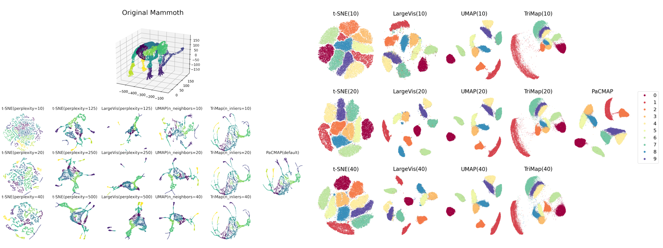
PaCMAP 성능을 단번에 보여주는 아래 사례 한번 보시고 아래에서 차근차근 알아가 보도록 하겠습니다 : )

 

Application of t-SNE, LargeVis, UMAP, TriMap and PaCMAP to the Mammoth and MNIST dataset

 

 

---

0. Dimension Reduction?!

해당 논문에서는 주로 시각화를 위한 툴로써 사용되는 차원 축소 방법론에 대해 이야기하고 있고, 딥러닝에서 많이 사용되는 representation과 같은 차원축소와는 (structure를 보존하지 못하고 정확한 시각화 못해서) 분리해서 설명하고 있습니다.

논문 제목에서부터 나와있는 t-SNE, UMAP과 TriMap에 대한 기본 개념과 한계점들을 살펴보면서 PaCMAP가 나오게 된 배경에 대해 살펴보겠습니다.

 

우선 시각화를 위한 차원축소 방법들이 가져야 한 중요한 특징이 있습니다. 원래 데이터의 local structure와 global structure를 잘 유지하면서 고차원에서 저차원으로 projection 해야 한다는 점입니다. 하지만 local str. 를 보존하는 것과 global str. 를 유지하는 것은 trade-off 관계에 있어서 둘 다 만족시키기 어렵다는 한계점이 있습니다.

• preservation of local/global str.에 대한 개념을 간단히 보면, local은 각 포인트들 간의 구조/이웃(가깝고 먼지)을 잘 유지하는 것이 목표이고 global은 이웃들/cluster들의 layout(구조)를 잘 유지하는 것이 목표라고 보면 되겠습니다.

local structure methods aim mainly to preserve the set of high-dimensional neighbors for each point when reducing to lower dimensions, as well as the relative distances or rank information among neighbors (namely, which points are closer than which other points).
Global methods aim mainly to preserve relative distances or rank information between points, resulting in a stronger focus on the preservation of distances between points that are farther away from each other

 

 

각 차원축소 방법들이 어떤 특징/한계를 보이는지 간단히 보면,

t-SNE

perplexity parameter에 민감해서 parameter 값에 따라서 가짜 cluster를 만들기도 하고 잘 만들기도 합니다. 그리고 local structure는 잘 유지하지만 global structure는 잘 유지하지 못한다는 한계가 존재합니다.

https://distill.pub/2016/misread-tsne/

How to Use t-SNE Effectively

 

UMAP

t-SNE와 마찬가지로 local structure는 잘 유지하지만 global structure는 잘 유지하지 못하고, PCA initialization에 의존도가 굉장히 높다고 합니다.

 

TriMap

triplet 모델인 TriMap은 t-SNE와 UMAP과 비슷한 local structure 유지 성능을 가지면서도 global structure도 잘 유지한다고 합니다. 하지만 가끔 local structure 유지에 어려움을 보이기도 해 다소 불안정한 성능을 보인다는 한계가 있습니다. 그리고 UMAP과 마찬가지로 PCA initialization에 의존도가 굉장히 높다고 합니다.

 

그렇다면 PaCMAP은 이러한 한계점을 극복하기 위해 어떻게 접근했고 해결했는지 이어서 알아보겠습니다.

 

 

1. PaCMAP, Pairwise Controlled Manifold Approximation Projection

Main Goal

is to understand what aspects of DR methods are important for preserving both local and global structure.

논문에서 소개하는 PaCMAP의 주목표는 local/global str. 를 유지하는데 차원 축소 방법론의 어떤 부분이 중요하게 작용하는지 이해하는 것이라고 했습니다. 저자는 (새로운 차원축소 매커니즘에 대한 이해를 바탕으로) local str. 유지를 위한 loss fuction에 여러 유용한 design principles을 제안하고 global str. 유지를 위해 어떤 요소를 유지할지 고르는(the choice of which components to preseve)것이 중요하다는 점을 찾아내었습니다.

 

Loss function

Loss function은 3개의 부분으로 나눌 수 있는데, Near pairs를 서로 가깝게하는 부분/ Mid-near pairs를 약하게 가깝게 하는 부분/ Further pairs를 멀게 하는 부분으로 구성되어 있습니다. 저자가 설명하는 youtube에서도 너무 간단하지 않냐며... 이게 전부라고 하셨습니다! ㅎㅎ

 

각 pair에 대한 정의는 아래와 같습니다.

• Near pair : 가장 가깝게 해야하는 pair, pair $i$ with its nearest $n_{NB}$ neighbors defined by the scaled distance
• Mid-near pair : 약하게 가깝게 해야하는 pair, For each $i$, sample 6 observations, and choose the second closest of the 6, and pair it with $i$
• Further pairs : 서로 멀리 떨어져야하는 pair, Sample non-neighbors

 

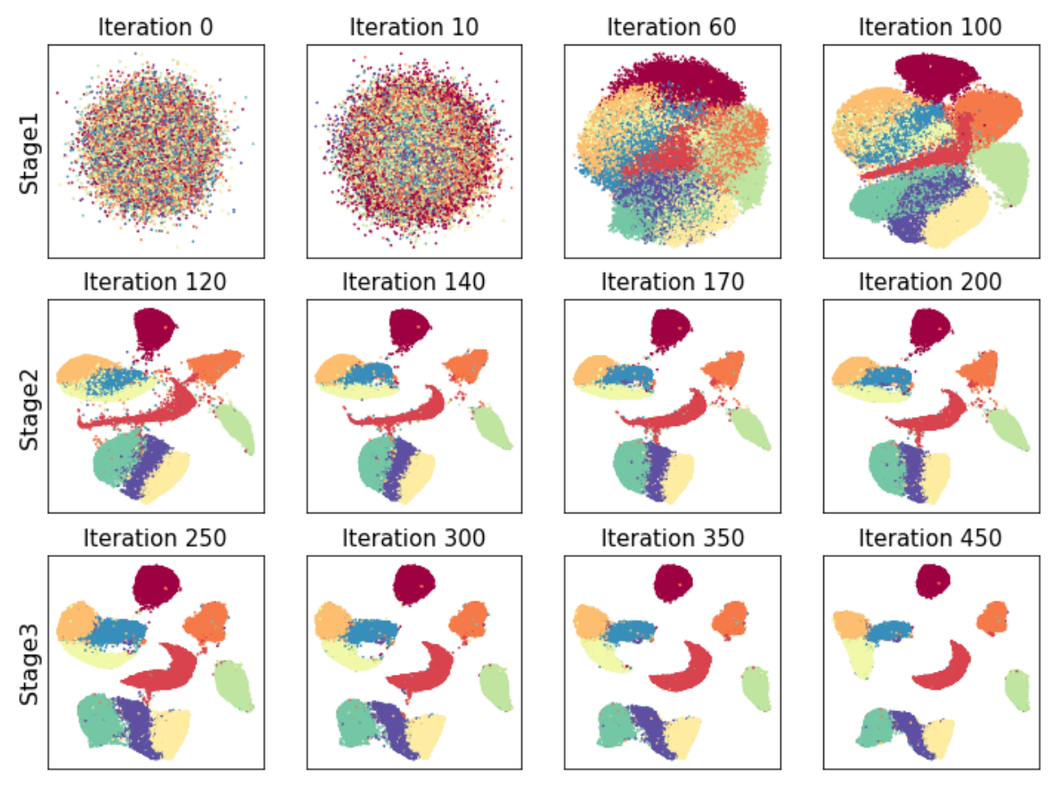
아래 Loss를 최소화하기 위해서 3가지 stage로 나눠 학습을 진행을 진행합니다. 각 stage별로 가중치를 달리해서 loss의 각 부분의 영향도가 매 stage마다 달라지고 그것들이 모여 local/global을 잘 구분하게 됩니다.

 

Loss를 최소화하는 방법은 아래 3가지 stage로 진행이 됩니다. 

In the first stage (i.e., the first 100 iterations of an optimizer such as Adam), set $w_{NB}=2$, $w_{MN}(t)=1000 - 3$, $w_{FP}=1$
In the second stage (iterations 101 to 200), set $w_{NB}=3$, $w_{MN}=3$, $w_{FP}=1$
In the third stage (iteration 201 to 450), $w_{NB}=1$, $w_{MN}=0$, $w_{FP}=1$

첫 번째 stage에서는 Mid-pair에 대한 가중치를 1000에서 3으로 줄여가면서 강하게 당겼다가 놓으면서, neighbor를 가깝게 하고, FP도 멀어지게 하면서 대략적인 str. 를 잡습니다.

두 번째 stage에서는 가까이에 있는 neighbors를 강하게 가깝게 만들려고 시도하면서 FP에 대해서도 멀게하도록 합니다.

세 번째 stage에서는 가까이에 있는 neighbors에 대한 미세 튜닝을 진행하면서 FP에 대해 멀어지게 합니다.

 

아래 MNIST 예제를 보면, Stage1에서 100번 iteration 되면 대략적인 구조를 파악하게 되고 Stage2에서 추가적으로 local str. 를 미세 조정하고 Stage3에서 local str. 와 global str. 를 추가적으로 조정해서 최종적으로 local/global str. 모두 잘 유지하게 됩니다.

 

Visualizations of the low-dimensional embedding over the three-phase optimization process of PaCMAP on the MNIST dataset. This figure demonstrates how phases 2 and 3 refine the local structure of the embedding.

 

Contributions

위에서 계속 봐왔지만, PaCMAP은 Local/Global str. 를 동시에 유지해 뛰어난 시각화 성능을 보이고, Computation time 측면에서도 강점을 보인다고 합니다.

 

 

 

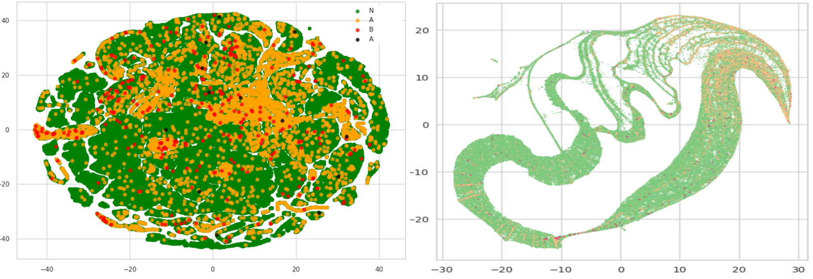
2. Application of PaCMAP

언제나 우리가 활용하기 좋은 kaggle의 credit card 데이터를 활용해서 PaCMAP의 성능을 살펴보겠습니다.

(...업데이트예정...)

왼쪽 : t-SNE/ 오른쪽 : PaCMAP

PaCMAP GitHub

https://github.com/YingfanWang/PaCMAP

GitHub - YingfanWang/PaCMAP: PaCMAP: Large-scale Dimension Reduction Technique Preserving Both Global and Local Structure

import pacmap
import numpy as np
import matplotlib.pyplot as plt

# loading preprocessed coil_20 dataset
# you can change it with any dataset that is in the ndarray format, with the shape (N, D)
# where N is the number of samples and D is the dimension of each sample
X = np.load("./data/coil_20.npy", allow_pickle=True)
X = X.reshape(X.shape[0], -1)
y = np.load("./data/coil_20_labels.npy", allow_pickle=True)

# initializing the pacmap instance
# Setting n_neighbors to "None" leads to a default choice shown below in "parameter" section
embedding = pacmap.PaCMAP(n_components=2, n_neighbors=None, MN_ratio=0.5, FP_ratio=2.0) 

# fit the data (The index of transformed data corresponds to the index of the original data)
X_transformed = embedding.fit_transform(X, init="pca")

# visualize the embedding
fig, ax = plt.subplots(1, 1, figsize=(6, 6))
ax.scatter(X_transformed[:, 0], X_transformed[:, 1], cmap="Spectral", c=y, s=0.6)